EpicWorldModel: Exploration-driven Planning with Latent World Models

Each point represents one predicted future, projected into a shared PCA space. Under high uncertainty, the futures are more spread out. In early planning steps when the goal is not in view, the future directions disagree, and the EpicWorldModel favors exploration. As the goal comes into view the future predictions collapse, disagreement drops, and the planner commits.

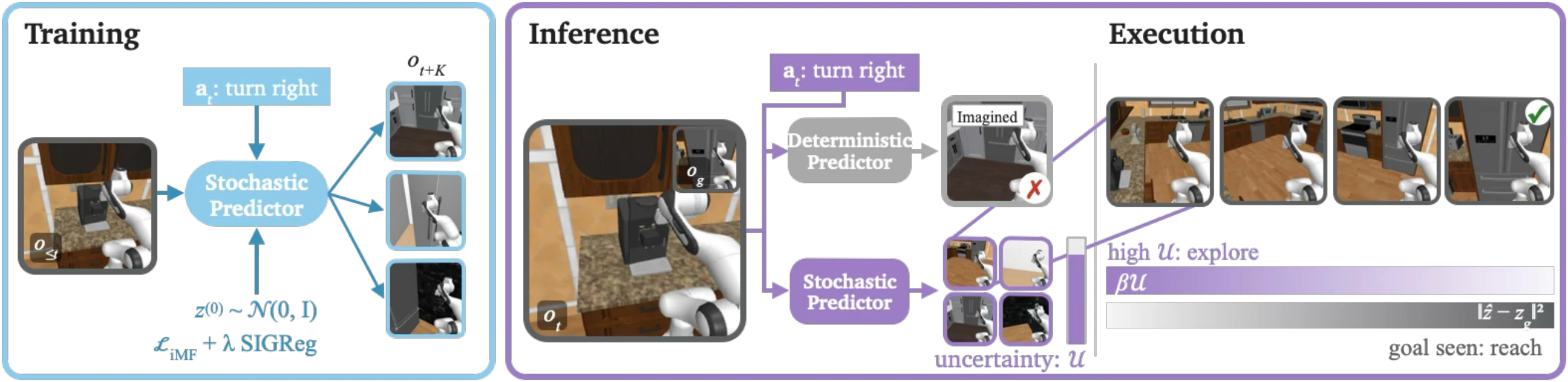
Assume a simple scenario: A robot is deployed in an unkown home and asked to navigate to a fridge that is initially out of view. A deterministic latent world model memorizes the location of the fridge from training data and commits early to a halucinated direction at inference time, even when the true location differs.

EpicWorldModel instead maintains a distribution over plausible futures. Where these futures disagree, the uncertainty is high and the planner explores different possibilities. Once the goal is partially in view, the futures agree and the planner commits to reaching it.

Summary Latent world models based on Joint-Embedding Predictive Architecture (JEPA) are deterministic by design. While successful in fully observable scenarios, this paradigm breaks down when past observations and actions lead to multiple plausible futures, e.g., due to occlusion. We introduce EpicWorldModel, a framework to train stochastic JEPAs for environments and tasks with inherent uncertainty under partial observability. We jointly train the EpicWorldModel predictor with its latent representation space to directly predict multiple potential future states using a flow-matching objective, when the goal-relevant scene content is absent from the conditioning history. We show that flow predictive variance, motivated by its relation to an upper bound on predictive entropy, serves as a useful exploration guidance for planning. By incorporating this uncertainty signal into Cross-Entropy Method (CEM)-based planning, our approach balances goal-reaching with exploration of uncertain regions where occluded goals are most likely to be located. We demonstrate the effectiveness of EpicWorldModel through a series of latent planning experiments with the best or on-par performance across tasks, showing an increase in success rate of up to about 22 points over LeWorldModel.

In RoboCasa NavigateKitchen, a mobile manipulator is asked to "navigate to the fridge" in unseen kitchen layouts. In the episodes above, the fridge starts outside the field of view or occluded by cabinets and counters. Guided by the uncertainty \(\mathcal U\), the robot first turns and moves toward unobserved regions of the kitchen, then commits to the goal once the fridge becomes visible.

EpicWM (FM) and EpicWM (iMF) denote EpicWorldModel trained with the flow matching and iMeanFlow objectives respectively, and \(\beta\) weights the exploration bonus. We compare against the deterministic LeWorldModel (LeWM), also with 3× more planning candidates (LeWM 3×). Two experiments vary how much of the goal is initially visible. First, we vary the robot's starting distance to the fridge, which correlates with initial goal visibility. With the same planning budget, the stochastic predictor alone (\(\beta=0\)) already outperforms deterministic LeWorldModel, and giving LeWorldModel 3× more planning candidates helps at short range but not at larger distances. The bonus helps most at long range, where the goal is hidden.

Second, we measure the fraction of the fridge visible in the first observation. When the goal is initially mostly hidden, exploration turns 1 of 6 successes into 5 of 6. When the goal is fully visible, the bonus is unnecessary.

We evaluate EpicWorldModel on five tasks with restricted fields of view: Visual PointMaze Giant, Visual AntMaze Giant and Visual Scene from OGBench, Car Racing from Gymnasium, and LabMaze from DMLab. We compare against goal-conditioned RL (GCIQL, GCIVL) and latent world models (PLDM, DINO-WM, LeWorldModel).

Success rates in % (orange: EpicWorldModel, blue: baselines). On Visual PointMaze Giant, EpicWorldModel improves success by about 22 points over LeWorldModel, and on Car Racing it nearly doubles LeWorldModel's success rate. On tasks with high-dimensional action spaces (AntMaze, Visual Scene) it performs on par with the baselines, suggesting that stochastic latent prediction helps most in partially observable tasks with relatively low-dimensional actions.

The Gaussian latent geometry induced by SIGReg gives the flow-matching objective two useful properties. Proofs can be expanded below.

Proposition 1 (Data-independent gradient noise). Given an isotropic Gaussian latent space \(\mathbb P_{\mathbf Z_t}=\mathcal N(0,I_d)\), for every flow step \(\tau\in[0,1]\) the excess variance of the conditional velocity target is

\[\mathrm{Var}\big(v_{\mathrm{tgt},\tau}\mid\mathbf z^{(\tau)}\big)=\frac{1}{(1-\tau)^2+\tau^2}\,I_d .\]

Gradient variance is therefore bounded and data-independent. For a general latent variance \(\sigma^2\), the same derivation gives \(\sigma^2/((1-\tau)^2+\tau^2\sigma^2)\), which peaks at \(1+\sigma^2\). Drag the slider to see how the noise would grow without SIGReg, which pins \(\sigma^2\approx1\) (gray curve).

Proof of Proposition 1

By the law of total variance applied to the conditional velocity target \(v_\text{tgt}=\mathbf z^{(1)}-\mathbf z^{(0)}\),

\[\mathrm{Var}(v_\text{tgt})=\mathbb E_{\mathbf z^{(\tau)}}\big[\mathrm{Var}(v_\text{tgt}\mid\mathbf z^{(\tau)})\big]+\mathrm{Var}\big(\mathbb E[v_\text{tgt}\mid\mathbf z^{(\tau)}]\big).\]

By independence of \(\mathbf z^{(0)}\sim\mathcal N(0,I_d)\) and \(\mathbf z^{(1)}\), with \(\sigma^2\) denoting the variance of the SIGReg-induced latent space, \(\mathrm{Var}(v_\text{tgt})=(\sigma^2+1)I_d\). Since \(\mathbf z^{(\tau)}=(1-\tau)\mathbf z^{(0)}+\tau\mathbf z^{(1)}\),

\[\mathrm{Cov}\big(\mathbf z^{(1)}-\mathbf z^{(0)},\mathbf z^{(\tau)}\big)=(\tau\sigma^2-(1-\tau))I_d,\qquad \mathrm{Var}(\mathbf z^{(\tau)})=\big[(1-\tau)^2+\tau^2\sigma^2\big]I_d .\]

The marginal vector field is the linear conditional expectation

\[v_\text{tgt}(\mathbf z^{(\tau)})=\frac{\tau\sigma^2-(1-\tau)}{(1-\tau)^2+\tau^2\sigma^2}\,\mathbf z^{(\tau)},\qquad \mathrm{Var}\big(v_\text{tgt}(\mathbf z^{(\tau)})\big)=\frac{(\tau\sigma^2-(1-\tau))^2}{(1-\tau)^2+\tau^2\sigma^2}I_d .\]

Subtracting,

\[\mathbb E_{\mathbf z^{(\tau)}}\big[\mathrm{Var}(v_\text{tgt}\mid\mathbf z^{(\tau)})\big]=(\sigma^2+1)I_d-\frac{(\tau\sigma^2-(1-\tau))^2}{(1-\tau)^2+\tau^2\sigma^2}I_d=\frac{\sigma^2}{(1-\tau)^2+\tau^2\sigma^2}I_d .\]

Because \((\mathbf z^{(0)},\mathbf z^{(1)},\mathbf z^{(\tau)})\) is jointly Gaussian, conditional variances are homoscedastic, so the identity holds for every \(\mathbf z^{(\tau)}\). Under SIGReg, \(\sigma^2\approx1\), which yields the result. \(\blacksquare\)

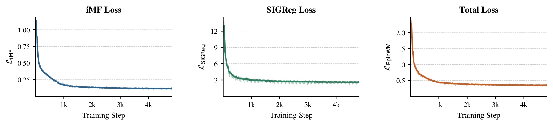
In practice, the losses of EpicWorldModel converge smoothly with little per-step variance, as Proposition 1 predicts:

Proposition 2 (Uncertainty as a conditional entropy upper bound). Sampling \(N\) noise seeds and running the predictor yields an ensemble \(\{\hat{\mathbf z}^{(1)}[i]\}_{i=1}^N\) with disagreement \(\mathcal U=\frac1d\sum_{j}\widehat{\mathrm{Var}}_i(\hat{\mathbf z}^{(1)}_j[i])\). For a well-trained predictor, \(\mathbb E[\mathcal U]=\mathrm{tr}(\Sigma_{\mathbf c_t})/d\), and by the maximum entropy theorem

\[H\big(\mathbf z^{(1)}\mid\mathbf x_t,\mathbf c_t\big)\le\frac d2\log\!\big(2\pi e\cdot\mathcal U\big).\]

Because the latent space is \(\mathcal N(0,I_d)\), \(\mathcal U\) has an absolute scale with \(0\le\mathbb E[\mathcal U]\lesssim1\): \(\mathcal U\approx0\) indicates a confident prediction, \(\mathcal U\approx1\) a prediction as diffuse as the prior. The bound is tight only for isotropic covariances, so we use \(\mathcal U\) as a practical exploration bonus rather than an entropy estimate.

Proof of Proposition 2

(i) Unbiasedness. For a well-trained \(\mathcal P_\varphi\), the ensemble members are i.i.d. draws from \(p(\mathbf z^{(1)}\mid\mathbf x_t,\mathbf c_t)\), so the sample variance of dimension \(j\) is an unbiased estimator of \([\Sigma_{\mathbf c_t}]_{jj}\). Averaging over dimensions gives \(\mathbb E[\mathcal U]=\mathrm{tr}(\Sigma_{\mathbf c_t})/d\).

(ii) Entropy upper bound. For a given covariance, the Gaussian maximizes differential entropy, so \(H(\mathbf z^{(1)}\mid\mathbf x_t,\mathbf c_t)\le\tfrac12\log\big((2\pi e)^d|\Sigma_{\mathbf c_t}|\big)\). Applying Jensen's inequality to the eigenvalues \(\lambda_j\) of \(\Sigma_{\mathbf c_t}\),

\[\frac1d\log|\Sigma_{\mathbf c_t}|=\frac1d\sum_{j=1}^d\log\lambda_j\le\log\Big(\frac1d\sum_{j=1}^d\lambda_j\Big)=\log\mathcal U,\]

with equality iff \(\Sigma_{\mathbf c_t}\propto I_d\). Hence \(|\Sigma_{\mathbf c_t}|\le\mathcal U^d\) and \(H(\mathbf z^{(1)}\mid\mathbf x_t,\mathbf c_t)\le\tfrac d2\log(2\pi e\cdot\mathcal U)\).

(iii) Bounded scale. By the law of total variance, \(\mathrm{Cov}(\mathbf z^{(1)})=\mathbb E[\Sigma_{\mathbf c_t}]+\mathrm{Cov}(\mathbb E[\mathbf z^{(1)}\mid\mathbf x_t,\mathbf c_t])\). With an isotropic Gaussian latent space, \(\mathbb E[\mathrm{tr}(\Sigma_{\mathbf c_t})]\le\mathrm{tr}(\mathrm{Cov}(\mathbf z^{(1)}))\approx d\), so \(\mathbb E[\mathcal U]\lesssim1\), with equality when the conditioning is uninformative. \(\blacksquare\)

Connection to expected information gain. Treating each noise sample \(\mathbf z^{(0)}\) as a "seed" of the world, the expected information gain of an action chunk is the mutual information between seed and future. Since the flow ODE is deterministic given its seed, the per-seed differential entropy is \(-\infty\) for every action chunk, so it does not affect which chunk has the highest EIG:

\[\begin{gathered}\mathrm{EIG}(\mathbf c_t)=I\big(\mathbf z^{(0)};\mathbf z^{(1)}\mid\mathbf x_t,\mathbf c_t\big)=H\big[\mathbf z^{(1)}\mid\mathbf x_t,\mathbf c_t\big]-\underbrace{H\big[\mathbf z^{(1)}\mid\mathbf z^{(0)},\mathbf x_t,\mathbf c_t\big]}_{=\,-\infty},\\ H\big[\mathbf z^{(1)}\mid\mathbf x_t,\mathbf c_t\big]\;\lesssim\;\frac d2\log\!\big(2\pi e\cdot\mathcal U\big).\end{gathered}\]

Maximizing \(\mathcal U\) therefore approximately maximizes an upper bound on the action-dependent part of the expected information gain.

Is the gain due to the exploration term, the stochastic predictor, or simply more compute? All results are on Visual PointMaze Giant unless noted otherwise.